Plant material
Samples of potato tuber were collected from two sources: (1) from Graminor’s core collection grown in field experiments at Ridabu, Norway, from 2019 to 2022, and (2) from a greenhouse inoculation experiment in which 840 interrelated potato lines were planted in sterile peat soil infected with a mixture of three S. europaescabiei strains from the NIBIO collection of plant pathogens (isolate nos. 08-12-01-1, 08-74-04-1, 09-185-2-1). In total, 7200 tubers of yellow and red genotypes were used. The core collection tubers represented different levels of infections naturally occurring in the field. Figure 1 shows four samples of tuber containing the full possible range of infections, from completely healthy to maximum severity.
Tile images were used as a training set for the deep learning process. The tiles correspond to a whole potato tuber. (A) and (C) correspond to a yellow and a red tuber respectively with no symptoms of common scab (CS); (B) and (D) correspond to a yellow and red tuber respectively with characteristics of severe CS infection, shown as brown spots and lesions on the skin. Scab symptoms can range from a few small lesions on the surface of the tuber to deep and open scab ulcers, covering most of the tuber surface.
Image acquisition
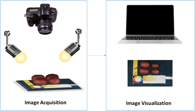
Tubers were washed, dried, and manually placed in groups of six onto a fiber blue background, along with a 5 cm ruler and a color scale palette for further analysis. Images were captured with a Canon PowerShot G9 X Mark II camera with a lens of 10.2–30.6 mm, 1:2.0–4.9, and a resolution of 20.1 megapixels. The camera was mounted on a Hama photo stand at a top-view angle of 40 cm from the target. The target was uniformly illuminated by daylight bulbs of 85W-5500 K. Camera settings were selected based on the best view of the tubers, ISO 1250, F-stop 1/125, exposure time 1/11, and focal length 10.2 mm. Digital images were stored in JPEG format with a pixel resolution of 7864 × 3648. The size of the tubers varies from 172 to 256 pixels in length. Figure 2 shows an illustration of the image acquisition protocol.

Diagram of the image acquisition protocol.
Database
The database contains 1100 images with 7154 yellow and red tubers. The tubers were categorized into five severity classes, with class 1 being healthy and classes from 2 to 5 that represent increasing severity levels of infection. The classes were attributed based on the area percentage of lesions on the potato tuber skin. A first approximation of the percentage of infected area was obtained in a semi-automated way, using the machine-learning tool Trainable Weka Segmentation (TWS)23 as a plugin for the software ImageJ24. Manual annotations of 200 images containing 1000 tubers were taken to train a random forest model25. The data was segmented into four classes (background, red tuber, yellow tuber, and scab). The segmentation was then taken to a pixel-wise classification where each pixel was classified as belonging to one of the four classes. This first quick approximation with color analysis was then corrected and validated manually.
Image and data processing
All the image processing was conducted using Python language26 with the package OpenCV (Open Source Computer Vision Library)27 for image manipulation and analysis of tuber morphology, and TensorFlow28 for the deep learning section; the algorithms developed were automated in a GUI (graphical user interface) that could be run over a single image or a large group of images as a batch.
GUI
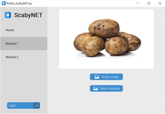
The GUI, hereafter called ScabyNet (Fig. 3), was developed in Python using the package Tkinter29 and customTkinter30. The GUI is user-friendly and contains two main modules and a tab designed as a home window. Modules 1 and 2, corresponding respectively to the estimation of tuber morphology traits and area lesions by CS.

The ScabyNet GUI application with all associated options and functions to evaluate potato tuber images.
Home
The home module contains information about the functionality of ScabyNet, where the user receives instructions on how to use the application.
Module 1: morphology features
The morphology module is a fully embedded data processing pipeline that estimates potato tuber morphology characteristics from color images. The module measures for each tuber, length, width, area, length-to-width ratio, circularity, and color values distinguishing between red and yellow tubers. The color analysis is performed in the L*a*b* color space: lightness, a*, and b* chromaticity values for respectively the green–red and yellow-blue axes31.
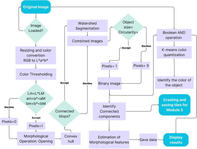
The steps in the processing chain of this module are presented in Fig. 4 and described in more detail in the following subsections and the flowchart in Fig. 5.

Workflow of the color-morphology module for features extraction, saving, and displaying results. (A) Original image to be processed; (B) binary image containing the desired and non-desired objects after resized, segmented, and filtered by morphology; (C) Identified connected components, non-convex blobs (red) and convex-blobs (green); (D) Processed image with segmented tubers.

Flowchart of the processing chain, operation algorithms, and outputs for the estimation of tuber morphology features.
Resizing and color segmentation
To remove the background, facilitate object identification, and decrease computation time, the image size was reduced from 4864 × 3648 to 1459 × 1094 pixels (one-third, conserving proportions). Then, a color conversion was applied from the RGB to the L*a*b* color space, using the features of the OpenCV package. This color representation was chosen because it was designed to approximate human psychovisual representation. A binary filter was applied to remove undesired objects. Each channel of the image was subjected to an examination to determine the adapted threshold. Subsequently, the resulting binary image was used as a mask for the original one.
Morphological operation: opening
Due to variations in lighting intensities, drops of shadows, and reflections, some objects in the image contained gaps. They were corrected with the flood-fill algorithm32, ensuring object integrity in the image. However, despite this correction of the gaps, some artifacts remained on the image. To discard them, a morphological opening operation was applied33. The opening consists of removing pixels on the object boundaries (erosion), then adding pixels to the new boundaries (dilation) on the resulting image. In both cases, the same 5 × 5-pixel square kernel was used as a structuring element. This structuring element identifies the pixel to be processed and defines the neighborhood of connected components based on this binary information. As a result of the opening, the small objects were removed from the image while the shape and size of the tubers were preserved.
Identifying connected blob components
Once the segmentation and color reduction was applied, the next step was to identify the tubers. In some cases, tubers were found to be placed too close to each other in the image. Thus, they were detected as a single component. A distinction between connected and disconnected components was performed based on convexity criteria to solve this issue. The operation works in two steps, finding contours, then computing their convex hull34. Convex objects i.e. individual tubers were copied and kept apart (noted image A) meanwhile objects corresponding to connected blobs, i.e., joint tubers (noted image B) were submitted separately to a segmentation process to split the connected blobs into the correct individual tubers.
Segmenting with watershed transformation
The image containing only the connected blob components (image B), was processed with watershed transformation to split the blobs into individual tubers and obtain the correct tuber count and morphology. The watershed transformation is based on topographic distances. It identifies the center of each element in the image using erosion, and from this point to the edges of the object, it estimates a distance map. Then, this area “topological map” is filled according to the gradient direction, as if it were filled with water. In this way, all connected components are separated (noted image C)35,36. Subsequently, image c was combined with image A to gather all the identified individual tubers in only one image (D).
Filtering by size and circularity
Once the objects were whole, the tubers were isolated from the non-targeted objects (ruler, color scale palette, genotype serial tag, etc.). For this purpose, a filter was first applied according to the object’s area and then according to the circularity based on Eq. (1) given by Wayne Rasband24. After inspecting the area of tubers and their circularity, the min and max values were determined. Only objects of an area between 11,000 px2 and 104,000 px2 and of circularity higher than 0.7 were retained.
Estimating morphology features
Tubers were identified and labeled with an ID, then for each one, the following parameters were measured: area, perimeter, length, width, length-to-width ratio, and circularity. Afterward, to provide a visual representation of the processed input image, the original image was masked with the results from the size and circularity filter, leaving only the tubers. The following formula was used to calculate circularity:
$$Circularity = \frac{{\left( {4{ } \times \pi \times { }area} \right){ }}}{{Perimeter^{2} }}$$
(1)
Identifying tuber skin color
The tubers contained a complex color spectrum corresponding to variations of the skin, buds, lenticels, mechanical damage, common scab symptoms, and other possible defects. To overcome this problem, color identification was performed using a K-means color quantization37, aiming both at facilitating the identification and reducing computation time. The process consists of reducing the number of colors in an image from 256 × 256 × 256 possible values in the 8-bit RGB color model to the desired number of colors but preserving the important information of it. In this case, three colors were selected, (background and the two considered colors for tubers). Based on these values (clusters), the centroids were determined. Then the color was determined, according to the minimum Euclidean distance between all the respective colors present in the image to the three cluster centroids. Several repetitions were performed until the centroid of clusters did not show changes and the distance between the centroids and the color objects was minimal while the distance between centroids was maximal. Subsequently, the image was segmented into three colors and an 8-bit value was given to the respective object, ‘0’ to the background, ‘1’ to the red tuber, and ‘2’ to the yellow tuber.
Displaying results
When analyzing an individual image the results are directly displayed on the screen. A window with the image containing only the previously labeled potato tubers, and another window with a table containing the estimations of morphology and color features. On the other hand, when selecting a batch of images, the results are saved in a folder named ‘Results’ in the same source directory given by the user. The folder contains the processed images with the potato tubers labeled and a CSV file with all the measurements linked to the respective IDs.
Module 2: common scab detection
Deep learning
The deep-learning module processes individual tiles of fixed size (172 × 172 pixels) representing an individual tuber. The tiles contain the segmented tubers without background, resulting from the morphology module’s output.
Convolutional neural network architecture
A benchmark including six common architectures of CNN was conducted to model and predict the severity level of scab infection: VGG16, VGG19, ResNet50V2, ResNet101V2, InceptionV3, and Xception. These architectures were developed for different object recognition applications, including plant and disease classification, and ranked among the best performing in the deep-learning challenges38. A table comparing their characteristics is described in Table 1.
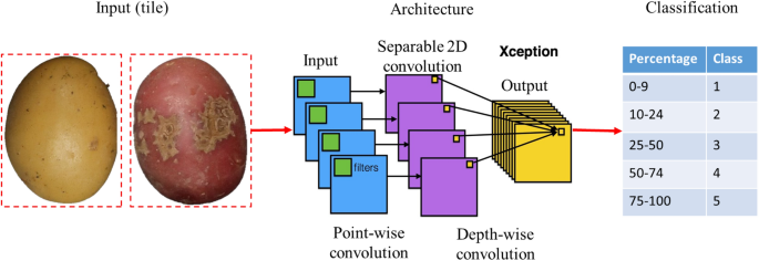
Different training strategies were compared and the training parameters were optimized according to the following criteria: minimizing the false positive rate of the infected classes in the health class and maximizing the separability between the minor and severe infection classes. The compared strategies were transfer learning and fine-tuning (Table 2). For both strategies, the networks are initialized with the weights resulting from the training on the ImageNet dataset containing 1.2 million images in 1000 classes such as “cat”, “dog”, “person”, and “tree”, among others39. In addition, we evaluated the robustness of the model with standard metrics (loss and accuracy). A schematic overview of ScabyNet-module 2 is shown in Fig. 6.

Schematic of module 2 for the detection and quantification of CS severity using deep learning with the ResNet architecture.
Generally, the complete training of a CNN is computationally intensive and requires a substantial amount of annotated data. These data are usually gathered from multiple collaborative projects. In the case of new applications, where less data is available, it is common to use a pre-trained network from public databases and adapt them to the specific application.
Visual inspections and manual measurements
Manual measurements for morphology traits
Tubers were measured manually using the ImageJ software24, using the 5 cm ruler placed at the bottom of the images as a scaling reference. Each potato was selected, and using the option “line” from the toolbox, the length and width were measured, then using these two parameters the length-to-width ratio was calculated.
Expert scores for disease severity of CS
The severity levels of CS are usually assessed visually and scored by an expert evaluating two parameters. First, the surface area covered with scab lesions, and second, the severity level, i.e., how deep the scab lesion is observed. The surface area covered is rated on a scale from 0 to 9, where 0 corresponds to no scab lesions on the surface, and 9 corresponds to about 100% of the surface area covered with lesions. The depth of the scab lesion is rated on a scale from 1 to 3, where 1 = superficial lesions, 2 = raised lesions, and 3 = deep lesions, the most severe coverage. Here, only the surface area was used and the expert scoring in ten grades (or severity classes) was transformed into a five classes severity scale.
Classes for CS
Potato tuber images were visually selected and classified in five classes, depending on the level of severity of CS on the surface area. Class 1 corresponds to 0–9%, class 2 to 10–24%, class 3 to 25–50, class 4 51–74%, and class 5 to 75%–100%. Figure 7, shows the scoring scale with corresponding images.

Images of the different severity levels of CS on yellow tubers. The rating of disease severity ranged from 0 to 100%. Scoring was based on the surface coverage of CS on the tuber.
Statistical analyses
Statistical analyses were performed using R version 4.146 and Python version 3.947. To evaluate module 1, the Pearson correlation coefficient was computed between the ground truth (manual measurements of the tubers), and the results obtained respectively with ImageJ and ScabyNet. For module 2, the two training strategies fine-tuning and transfer learning were compared. To ensure the reliability of the benchmark, the dataset (7154 potato tubers) was split into training, validation, and testing sets. By employing the function “Random Split” from Scikit Learn48, the main dataset was fractionated into 70% for the training set and the remaining 30% as a testing set. Subsequently, the training set was divided again using the same function to perform cross-validation, into 70% for the training set and the remaining 30% as a validation set. The results were compared with expert scoring in order to verify the accuracy of module 2.
Research involving plants
All the methods employed regarding plant materials followed the strict rules of the Swedish Agricultural University which are in accordance with all international standards, including those in the policies of Nature.


:max_bytes(150000):strip_icc()/ga_56946eb2ede4a68b_spcms-2000-ca7f9e9f55e442a3a9cdbbe530942db7-5aaaed2cbd0143a5ba007ae183d0131a.jpeg?w=768&resize=768,0&ssl=1)

